
holly ahit open source drawing
Free and open-source baby, powered by CC BY-NC content license
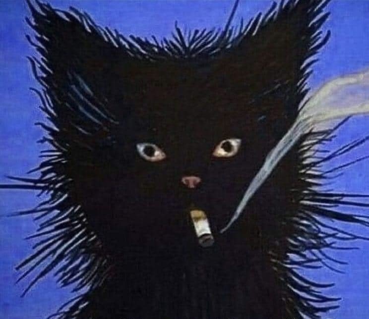
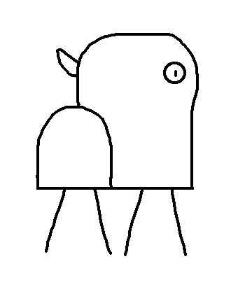
I used the default photos app on my phone to draw a totally normal cow

So I took your image and
ruined my MATLAB accountused the most normal part of your totally normal cow as a 3D [1]cockvolutionconvolution kernel. So in some sense, I dragged the red and purple part all across your image and added up the results. Here’s the result:
Here’s the MATLAB code:
normal_image = imread(“totally_normal_image.png”);
feature=normal_image(272:350,205:269,:);
feature_expansion = padarray(feature,[0,ceil((79-65)/2),0],‘replicate’);
for m = 1:1:3
new_normal_image(:,:,m) = conv2(normal_image(:,:,m),feature_expansion(:,:,m));

new_normal_image(:,:,m) = new_normal_image(:,:,m)/max(max(new_normal_image(:,:,m)));
end
imshow(new_normal_image)
[1] The original image was practically grayscale, so only a 2D convolution is required, i.e. over 2 spatial dimensions. Since you added color, it adds a extra dimension, one per color channel. Which makes it more annoying to work with in MATLAB. I mean, I could have just dumped everything into grayscale, but I need practice with processing color images anyways.
This is so f’n weird, I love it
Is that supposed to be a blood on the bottom right?
I think it’s a little more nsfw
Hold on this is gonna take some time but I might just try this and post in a few weeks
Now we wait and see what I come up with
I will watch your progress with the great interest
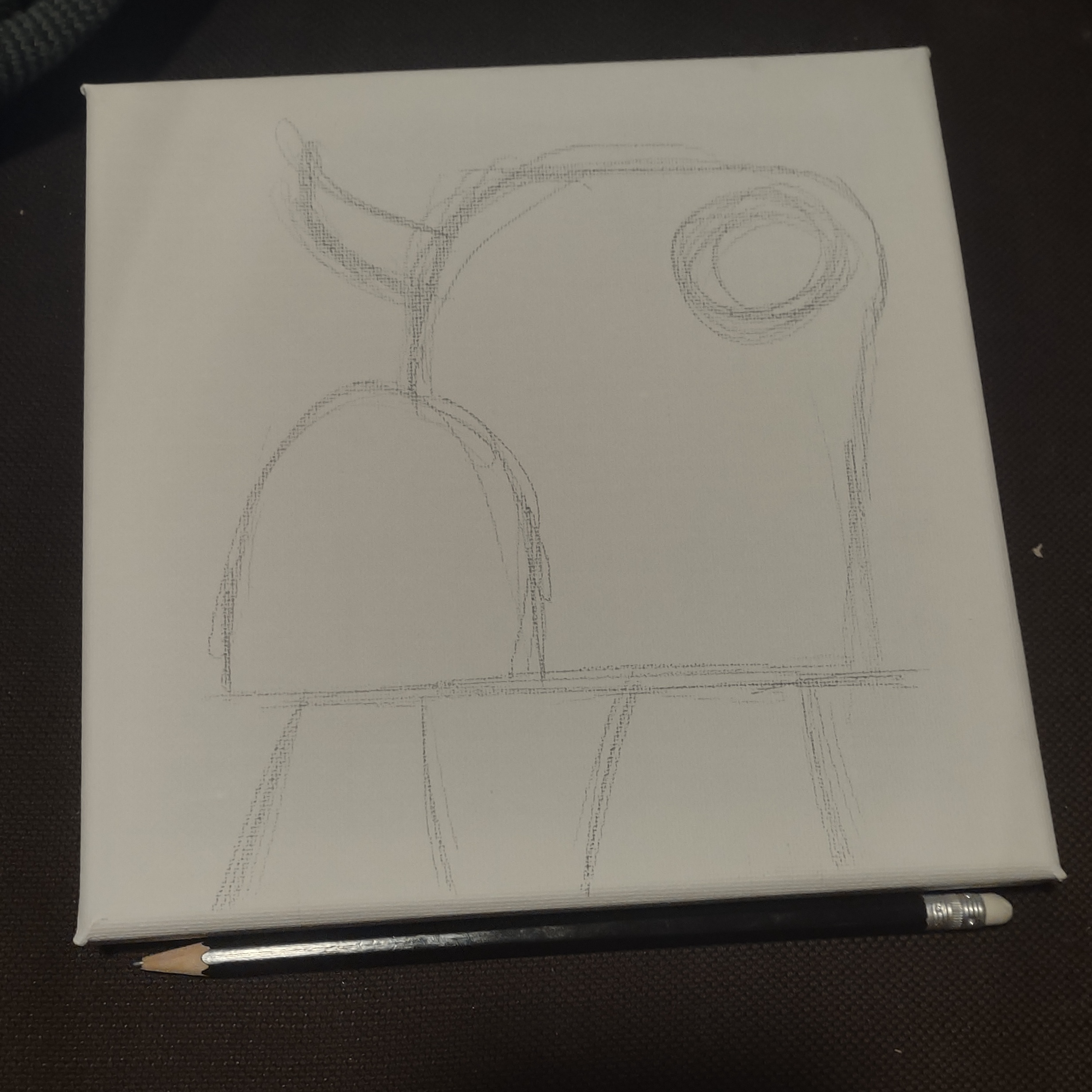
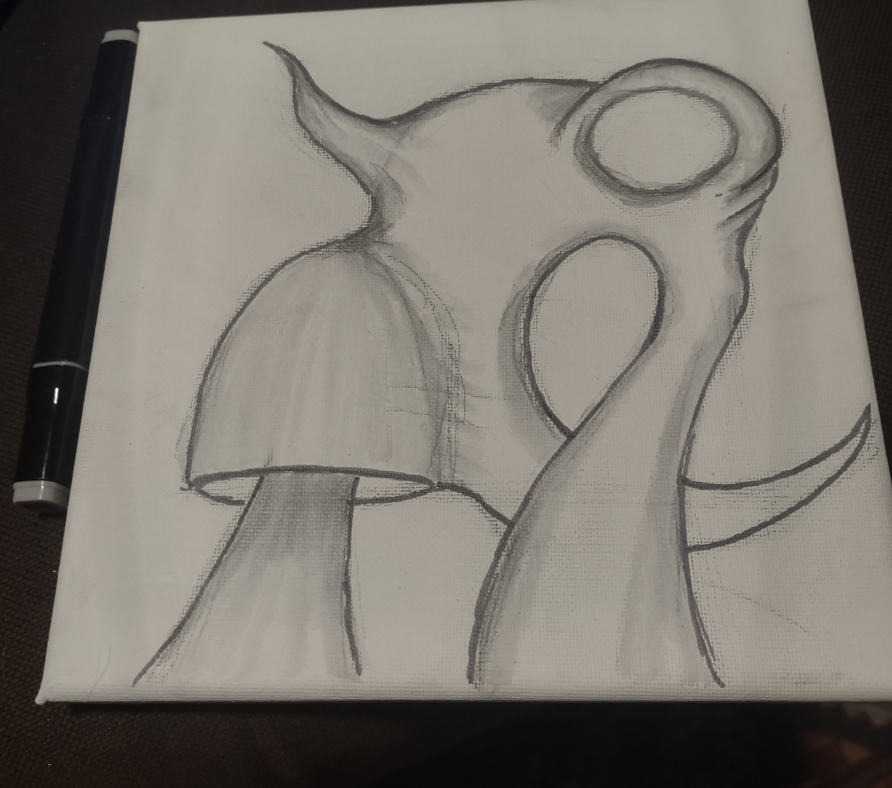
Okay hold on; I did it in a few hours, not weeks but it gets freaky fast:
-
Played around with the lines; erasing a few bits and rounding off some corners.
-
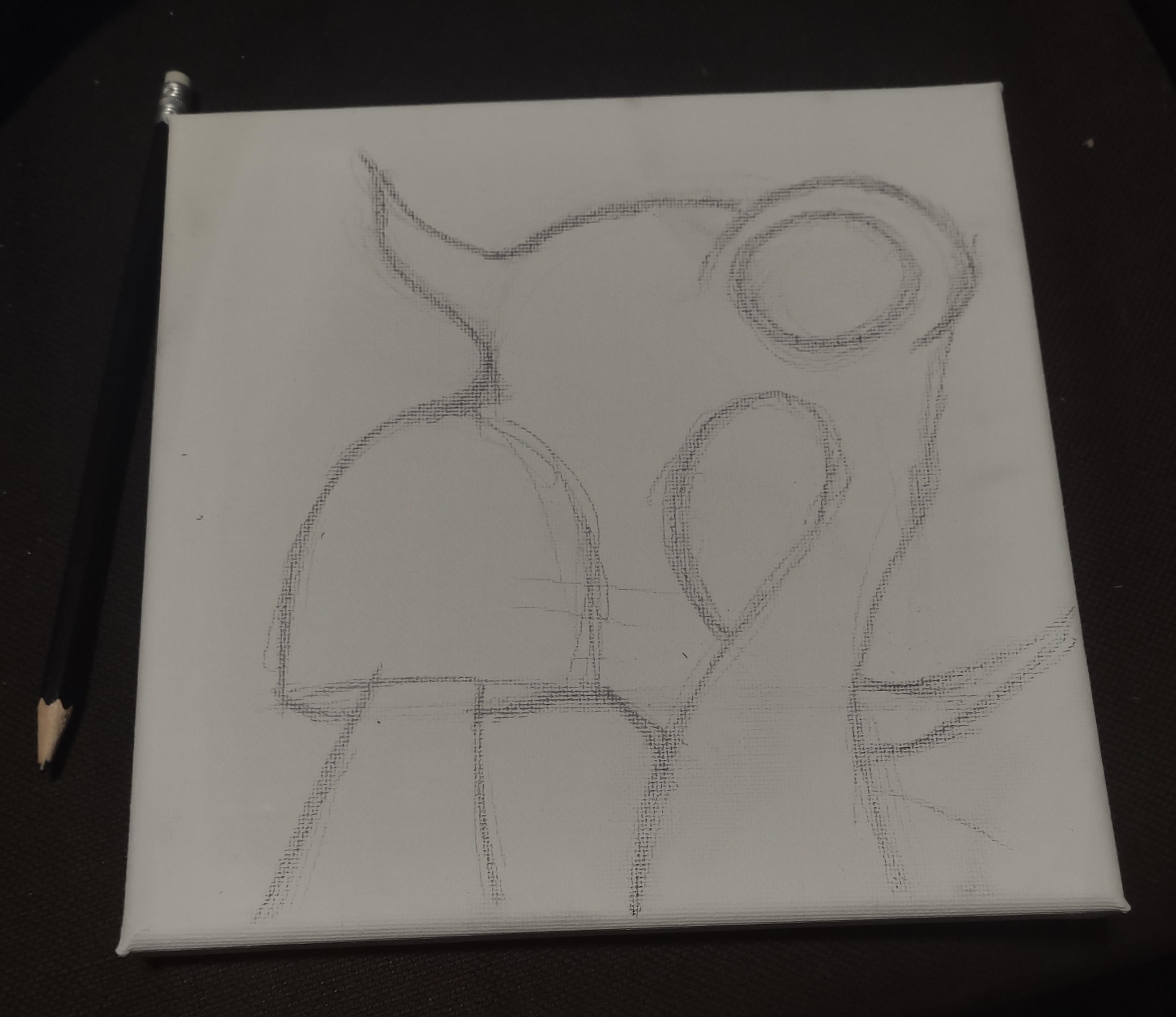
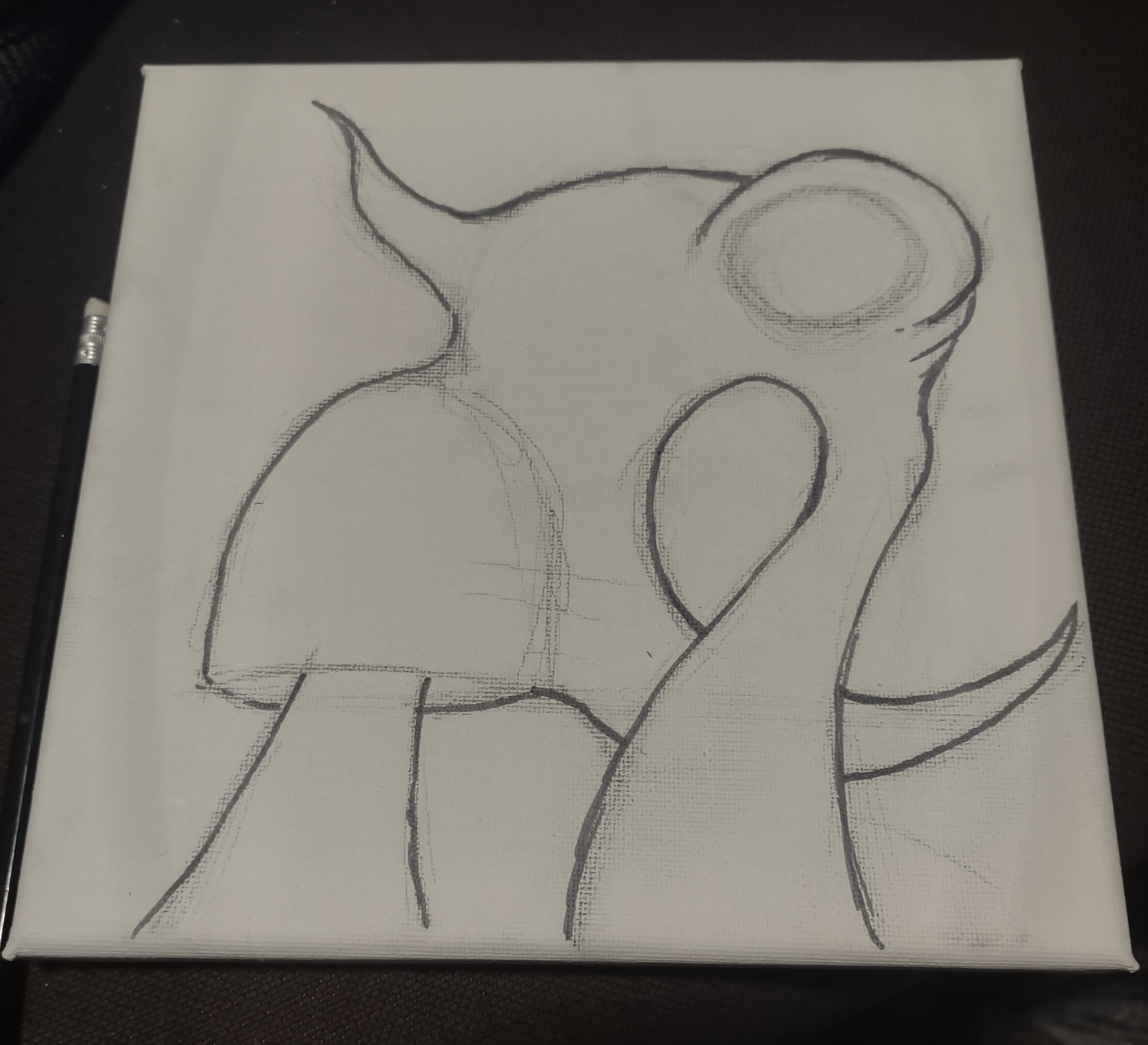
Did the outlines in marker
-
First bit of shading
-
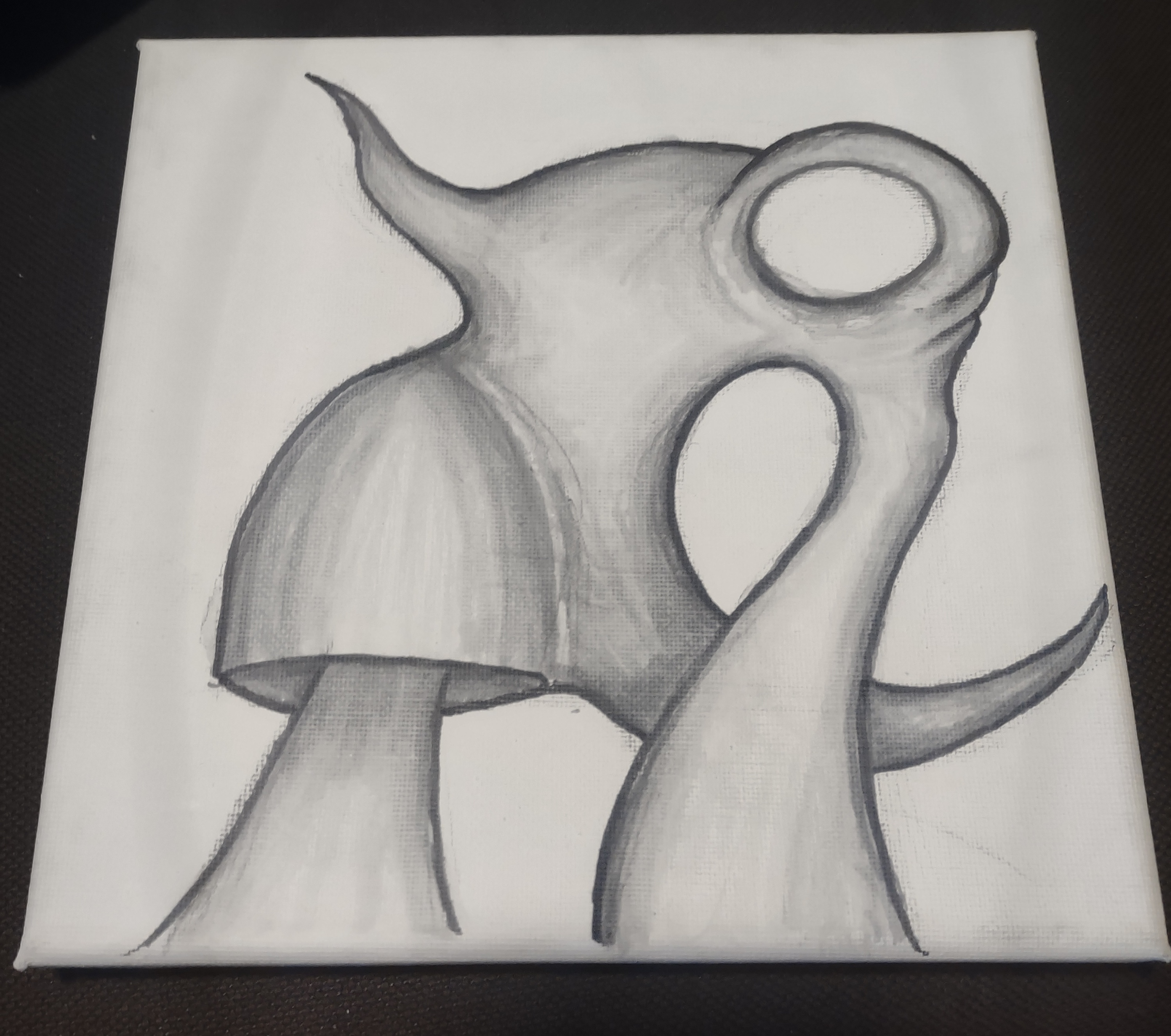
Left it overnight. Came back today and started building up the shades and lines

-
Bit more

-
Bit more and now I think I’m done.
-

over 9000 hours on paint
spoiler
.net
9000 hours well spent
I created this on my phone in MATLAB. You can probably do this in Octave with similar or the same code.
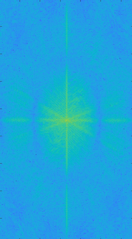
First, I downloaded the image from Lemmy, then uploaded it into my MATLAB app. I renamed the image to image.jpg, then ran the following code:
image=imread(“image.jpg”) imagesc(log10(abs( fftshift(fft2(image)) )))
fft2 applies a 2D Fast Fourier transform to the image, which creates a complex (as in complex numbers) image. abs takes the magnitude of the complex image elementwise. log10 scales the result for display.
Then I downloaded the image from the MATLAB app, went into the Photos app and (badly) cropped out the white border.
Despite how dramatically different it looks, it actually contains the same [1] information as the original image. Said differently, you can actually go back to the original with the inverse functions, specifically by undoing the logarithm and applying the inverse FFT.
[1] Almost. (1). There will be border problems potentially caused by me sloppily cropping some pixels out of the image. (2). It looks like MATLAB resized the image when rendering the figure. However, if I actually saved the matrix (raw image) rather than the figure, then it would be the correct size. (3) (Thank you to @itslilith@lemmy.blahaj.zone for pointing this out.) You need the phase information to reconstruct the original signal, which I (intentionally) threw out (to get a real image) when I took the absolute value but then completely forgot about it.
Can guarantee OP didn’t expect this when he was making the post, damn
I mirrored the image and added scanlines

This could be a logo for a hacker group or a scene group
No, you gave it a dump truck